| Presented in Partnership with: | |||
 |
|||
Rinsing Manual
Appendix D: Estimating Potential Dragout Reduction from Extended Drip Time
This section describes how to use measurements of the volume of solution draining from a rack of parts, sampled over successive time intervals, to estimate how much additional solution would have drained if drip time were extended. The drip rate decreases continuously over time, so some knowledge of the shape of the curve of drip rate vs. time is essential in order to calculate from the measured volumes what drip volume would be expected over some future time interval. A set of curves reproduced in an EPA report (see p. 25 in report) provides a set of drip rate vs. time curves for a typical plating solution (unspecified in the report). In the following section, a formula is developed which matches the shapes of the typical curves, and provides the basis for the estimate.
The shape of the curve:
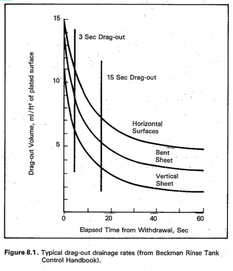
The chart from the EPA report, figure 9 in the text, is reproduced below:
|
|
Reproduced from Meeting Hazardous Waste Requirements for Metal Finishers, EPA/625/4-87/018, September 1987. |
Plots of dragout volume (volume of solution still clinging to rack) vs. time are provided for three different surface orientations (horizontal, vertical, and an intermediate case). The curves begin with a rapid decrease in dragout volume, with the rate of decrease becoming smaller until the curve flattens out. This is qualitatively the kind of behavior that would be expected if the drip rate were proportional to the amount of solution still on the rack. The curve would then have the form of an exponential decay,
dragout = Vstart * e-k*t + Vend
where Vstart, k, and Vend are constants. Specifically,
- Vstart is the dragout volume on the rack at time t = 0,
- k is the rate constant, which determines how rapidly the curve flattens out with time,
- Vend is the solution that remains on the rack after arbitrarily long times.
The exponential decay curve applies in a wide variety of situations, but the case of dragout volume is apparently not so simple. An exponential curve fitted to the first few seconds of the curve will not match the rest of the curve, and vice versa. However, a very close match can be obtained by adding two exponentials, with individual initial volumes and rate constants:
dragout = Vstart1 * e-k1*t + Vstart2 * e-k2*t + Vend
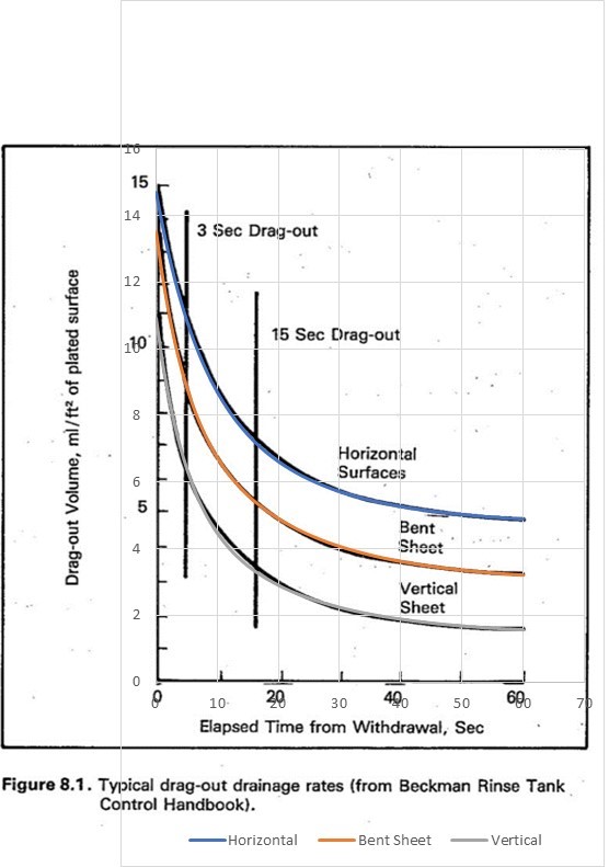
These curves were plotted on a spreadsheet, with the size of the grid adjusted to match the curves in the EPA report. The spreadsheet curves are shown below, superposed on a screenshot of the EPA report curves:
|
| Above curves overlaid with spreadsheet plots. |
The values of the parameters that provide this fit are:
| parameter | horizontal | bent sheet | vertical | units |
| Vstart1 = | 5 | 5 | 5.2 | ml/ft2 |
| k1 = | 0.15 | 0.22 | 0.22 | 1/sec |
| Vstart2 = | 5 | 5.5 | 4.3 | ml/ft2 |
| k2 = | 0.055 | 0.055 | 0.055 | 1/sec |
| Vend = | 4.7 | 3.0 | 1.4 | ml/ft2 |
The volumes are expressed in milliliters per square foot of surface area, to match the units used for the EPA report curves. The rate constants can be expressed simply as "percent per second", since for any single exponential decay curve, where the amount lost is proportional to the amount remaining, a constant percentage of the remaining weight will be lost every second. In this case, where two exponentials are being added, the percent in each case refers to the initial volume for that exponential.
For example, for the case of the vertical sheet, the total dragout volume left on the rack after the first second will be
e-0.22 * 5.2 = 4.17 ml/ft2 from the first term, plus
e-0.055 * 4.3 = 4.07 ml/ft2 from the second term.
After the next second, the remaining dragout volume will be
e-0.22 * 4.17 = 3.35 ml/ft2 from the first term, plus
e-0.055 * 4.07 = 3.85 ml/ft2 from the second term.
and so on for each subsequent second. (Note where the boldface terms in the first pair of equations show up in the second pair. The same pattern repeats every second.)
In other words, the model behaves as if there are two separate exponential decays occurring, each starting with its own initial volume of solution. For one of the components, the remaining volume at any point in time will be e-0.22 = 80.3% of what it was one second before, or equivalently, it loses 19.7% of its volume every second. For the other component, the corresponding percentage will be e-0.055 = 94.6%, or a loss of only 5.4% of its volume per second. The total dragout volume seems to consist of one portion that drips off relatively quickly, and a second portion that drips more slowly. After a long time, both of those exponentials will have decayed to nearly zero, leaving a third portion still on the rack that remains constant. (The other surface orientations have different parameter values, but the behavior is similar.)
This is consistent with the interpretation that some portion of the initial dragout volume is subject to bulk flow (Vstart1), another portion is strongly influenced by surface forces (Vstart2), and a third portion will remain clinging to the surfaces and never drip off (Vend). In practice, there wouldn't be sharp boundaries between layers, but the close agreement between the model and the measured curves suggests that a three-layer model is sufficient to produce a good estimate.
Using the model:
The specific numerical values found above for the rate constants k1 and k2, and the initial volumes Vstart1, Vstart2, and Vend that match the curve, cannot be carried over directly to plating solutions other than the particular solution used for the curve reproduced in the EPA report, tested under the conditions used when the curve was measured. (This information is not provided in the EPA report, and the publication from Beckman Instruments in which the curves originally appeared is not available.) Solutions with a different viscosity from the solution tested for the measured curves will, according to the model, obey the same equation, but with different values for the rate constants and initial volumes. The parameters will also depend on any additional factors, such as solution temperature, which affect the viscosity.
The model requires five parameters. One of them, Vend, does not enter into the calculation -- as far as the drip is concerned, it behaves as if it were part of the rack. That leaves two rate constants, and two initial volumes.
The values for the remaining four parameters that are appropriate to the plating solution being tested can be determined by a series of measurements. Each measurement involves collecting the amount of water dripping from the rack over a time interval. Measurements over four different time intervals are sufficient to determine the four parameters. In situations where it is impractical to sample four intervals (for example, if the racks are being sampled during production runs and the process cannot be interrupted) it is possible to obtain a reasonable estimate with as few as two values -- see the section "Estimating with two measurements" below for details.
Calculation details:
Each measurement involves determining the volume of solution that drips off the rack over a specific time interval. That volume, according to the model, will equal the difference between the values of the model equation for the times in seconds of the end and the beginning of the sampling interval. (Since we are only interested in the difference in dragout volume for two different values of t, the Vend term will cancel out of the difference, and will not be considered further.) The equation for the difference is:
dragout difference = Vstart1 * (e-k1*t1 - e-k1*t2) + Vstart2 * (e-k2*t1 - e-k2*t2)
where t1 and t2 are the start and end times, in seconds, of the sampling interval, measured from when the rack is raised above the tank.
To apply the equation to the measured drip volume samples, note that the left hand side of the equation is equal to the volume collected during each sampling interval, a known quantity. The right hand side is a function of the four unknown parameters and the known values of the start and end times for each measurement. Using the equation for one measurement, one of the parameters can be expressed in terms of the other three. The second measurement can then be used to eliminate a second parameter, and so on. After four measurements, all parameters have been determined. (Note that the sampling intervals must be independent, with different start and stop times, for the equations to be independent.) The equation then gives a fixed prediction for every start and stop time. If more than four measurements are available, the additional measurements serve as a check on the validity of the model.
Estimating with two measurements:
In practice, when sampling an ongoing process without interruption, it may only be feasible to sample two time intervals, one while the rack is over the plating tank, and one after it has moved over the first rinse tank, before it descends. It is possible to obtain an estimate from the model even if only two samples are available. Since there are four unknown parameters in the model, two additional assumptions must be introduced that will express two of the parameters in terms of the other two. Two pieces of input data will then be enough to determine the two remaining parameters.
The assumptions used for this calculation are: (1) that the ratio between the bulk and surface rate constants remains about the same as the viscosity changes, and (2) that the same is true for the ratio between the amount of bulk phase and surface-influenced phase volumes on the rack immediately after it has been fully withdrawn from the bath. (The exact start time is not critical, as long as it is consistent for all samples. The shape of the curve will be the same for whatever time is chosen as the starting point, as long as the rack has been pulled all the way out of the bath.)
The assumptions are valid as long as the bulk and surface phases respond similarly as the viscosity changes. For instance, if the viscosity of the solution decreases just enough to raise the bulk drip rate by ten percent, the model assumes that viscosity decrease has about the same effect on the surface-influenced drip rate as on the bulk, raising it also by ten percent. Taking the ratio of the two rates produces a fraction where both numerator and denominator increase by ten percent. When the ratio is expanded out in a power series, the ten percent increase in the ratio coming from the numerator will be canceled by a minus ten percent term coming from the denominator. The next term in the power series, involving the square of the percentages, will only affect the value of the ratio by ten percent squared, or one percent. So even if both the bulk and the surface rates change significantly, the ratio will change much less. The same argument applies to the ratio of starting volumes for the two phases.
Each of the two measured sample volumes can now be used as the left hand side of the dragout difference equation. The schematic form of the equation set is:
VP = Vstart1 * A + Vstart2 * B
VR = Vstart1 * C + Vstart2 * D
where VP and VR are the plating and rinse tank sample volumes, and A, B, C, and D are differences of exponential terms, as in the dragout difference equation written out above. This equation set can be inverted to express the unknown starting volumes in terms of the known sample volumes and the (still undetermined) coefficients:
Vstart1 = (- VP * C + VR * A) / (A*D-B*C)
Vstart2 = (VP * D - VR * B) / (A*D-B*C)
The ratio of starting volumes can then be expressed as:
Vstart1 / Vstart2 = (- VP * C + VR * A) / (VP * D - VR * B)
The left side of the equation is assumed to be equal to the value found in the EPA report data. The right side depends on the sampling times, which are known, but also on the rate constants, which have not yet been determined. Only one rate constant needs to be determined, since the model assumes that the ratio between the rate constants is equal to the ratio found in the EPA report.
The unknown rate constant can be determined numerically, by substituting a range of possible values for it into the equation, and choosing the value that gives the closest result to the known starting volume ratio. A spreadsheet that performs the calculation is available for download at STERC (http://www.sterc.org/files/xls/dripcalc.xlsx).
With all parameters determined, the model now predicts how much plating solution will drip off the rack over any given time period. In particular, it is easy to determine how much of the plating solution which is being dragged out into the rinse tank under current conditions would have been returned to the plating tank if the rack were to stay over the tank for a given number of seconds longer.
Note that the model is intended to provide reasonable estimates for plating solution flowing freely from part and rack surfaces. If solution is being retained in shallow pools on the rack, as might be the case for poorly racked parts, or in pockets of peeling rack coating, the drainage rate would depend on the shape of the pocket, with no guarantee of exponential behavior. This condition would be addressed by improved racking of parts, or better rack maintenance, rather than longer drip time.
The model provides the raw number of gallons of solution that the extra drip time would keep out of the waste stream. That is the fundamental piece of data for calculating waste treatment requirements, but it is still a step away from the number that answers the most significant question for cost-benefit evaluation: how will the avoided waste affect waste treatment costs? If parts racking and rack maintenance issues have been addressed, the model can be used to assess the expected percent reduction in waste treatment costs. The spreadsheet provides that number for an overall assessment, as well as a table showing how much solution will have dripped after each second, for more detailed calculations.
Even if solution is flowing freely from all surfaces, the improvement resulting from extra drip time will still be limited by the amount of solution that adheres to the surface. The EPA report indicates that for the reference ("bent sheet") surface orientation curve, of the 13.5 ml/ft2 of solution originally on the rack when fully withdrawn, the drip curve levels out with 3.5 ml/ft2 of solution still clinging to the rack (that is the amount measured by Vend above). In other words, 3.0/13.5 = 22% of the dragout remains unavoidable, and will continue to add to the treatment cost. The formula used on the spreadsheet for estimating potential savings includes the "unavoidable" dragout, so that the reduction is based on current treatment costs. But note that, if measured as a percent of "avoidable" dragout, extra drip time looks a lot more effective than the cost reduction percentage would suggest.
 |
 |
 |
The information contained in this site is provided for your review and convenience. It is not intended to provide legal advice with respect to any federal, state, or local regulation.
You should consult with legal counsel and appropriate authorities before interpreting any regulations or undertaking any specific course of action.
Please note that many of the regulatory discussions on STERC refer to federal regulations. In many cases, states or local governments have promulgated relevant rules and standards
that are different and/or more stringent than the federal regulations. Therefore, to assure full compliance, you should investigate and comply with all applicable federal, state and local regulations.